How Kimi K3 Engineered Its Way to the Frontier

Design · Kimi Delta Attention, balanced Mixture-of-Experts routing, and microVM infrastructure behind a 2.8T-parameter open-weight model

Kimi K3 is an open-weight model with 2.78T total parameters, 104B activated per token, and a 1M-token training context. The weights are on Hugging Face. Moonshot reports 88.3% on Terminal-Bench 2.1 against GPT-5.6 Sol’s 88.8%, 42.0% on SWE-Marathon against Claude Fable 5’s 35.0%, and the top score on BrowseComp at 91.2%. The independent numbers are in the same range. Artificial Analysis scores K3 at 57.1 on its Intelligence Index v4.1, fourth of 580 models, behind Claude Fable 5 at 59.9 and GPT-5.6 Sol at 58.9 and ahead of Claude Opus 4.8 at 55.7. No other open-weight model is close, with GLM-5.2 the next one at 51.1.

The 47-page technical report spans architecture, data, training, serving, and evaluation. This post covers three parts of it. The first is an attention design that reduces the cost of 1M-token contexts. The second is the kernel and parallelism work that makes that design fast enough to train at 3T scale. The third is agentic RL inside 51 million microVM sandboxes, paid for by the compute the first two saved. The code for all three is public.

• FlashKDA, CUTLASS kernels for the new attention

• MoonEP, expert-parallel MoE communication with perfect load balance

• AgentENV, the microVM sandbox runtime behind the RL training

One 128×128 matrix instead of a per-token KV cache

K3 replaces most of its attention layers with Kimi Delta Attention (KDA), a linear attention variant whose per-head memory is a fixed-size matrix instead of a growing key-value cache.

How softmax attention works

Every attention layer projects each token’s hidden state into three vectors. The query q_t is what the token seeks, the key k_t is what it offers, and the value v_t is what it contributes when matched. Three weight matrices, W_Q, W_K, and W_V, produce these vectors. Backpropagation trains the matrices, and every token multiplies its hidden state by the same three to get its own q, k, and v. q and k must have the same length because their match is a dot product, while v can have a different length. To produce one token’s output, attention scores its query against every key up to that token, applies a softmax to the scores, and returns the weighted sum of the values.

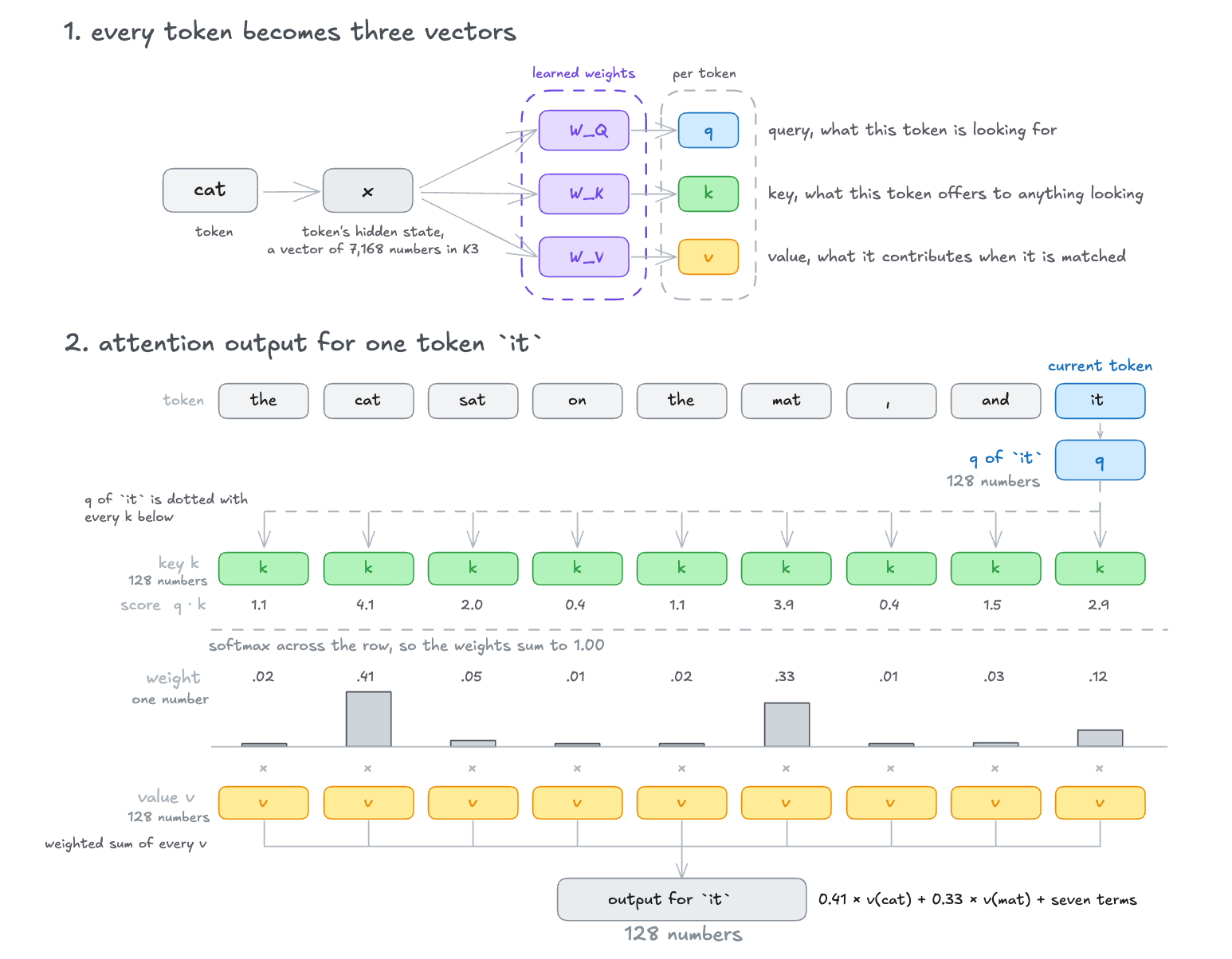
The diagram above shows one q, k, and v per token. A layer runs several heads side by side instead, each with its own W_Q, W_K, and W_V and its own private store. Per-head memory means what one head holds, so a layer has one store per head.

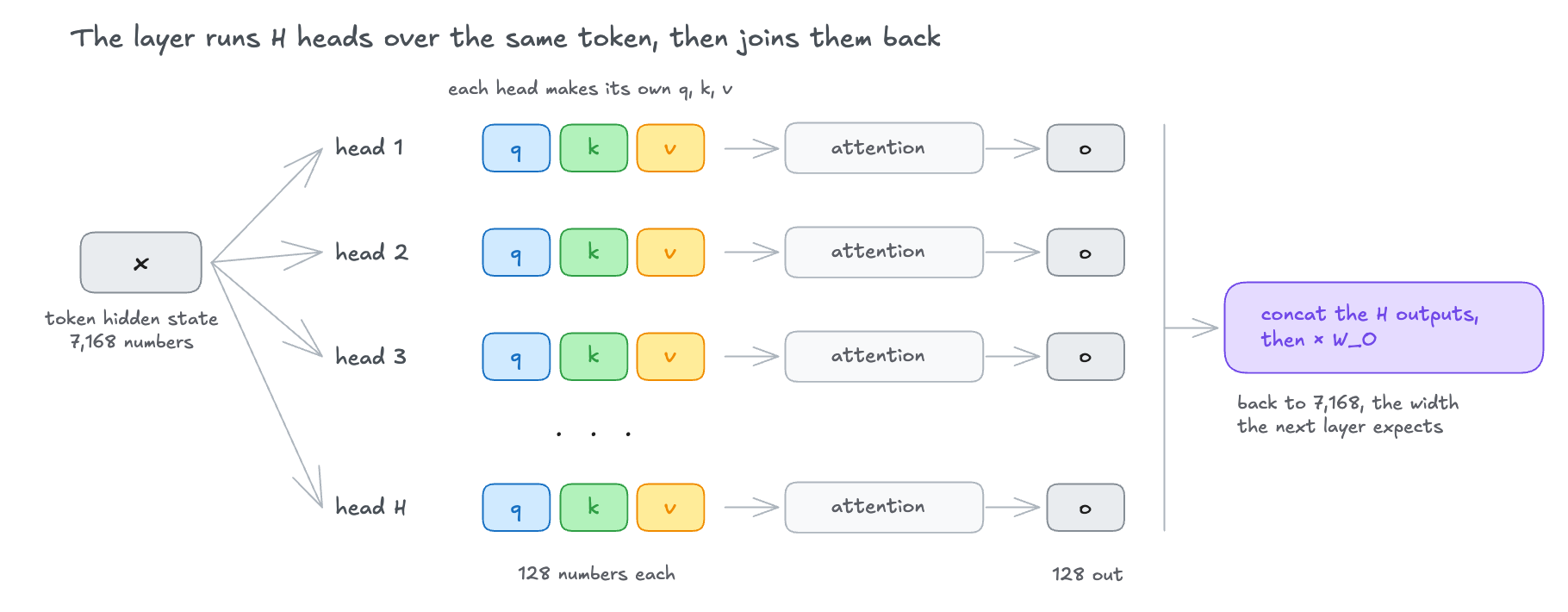
Every head reads the same 7,168-wide hidden state and projects it down to its own 128-long vectors. The layer runs the H heads independently, concatenates the outputs, and projects them back to 7,168.

Long contexts are expensive in softmax attention for two reasons.

First, the keys and values must stay in memory. Every new token scores its query against each earlier key and sums the matching values, so it rereads earlier keys and values. Recomputing them would require rerunning W_K and W_V over the sequence for every token. Instead, the model computes each one once and keeps it in the KV cache. The cache holds one key and value per token, head, and layer for the whole sequence. It grows with every token, so a 1M-token context carries a million entries in every layer. Any earlier token may match the current query, so none can be dropped.

Second, the work for one token grows with the number of tokens before it. The attention sum runs over every earlier position, so token 1,000 scores its query against 1,000 keys and sums 1,000 values, while token 1,000,000 does the same over a million.

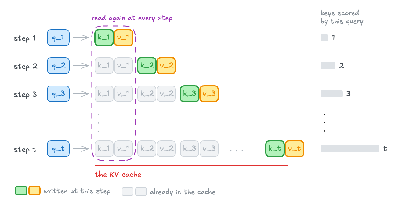
Each step writes one key and one value, shown in color, and reads back every gray pair from the steps before it. The cache grows because every pair it holds is still in use, and the bars on the right show how many keys each step has to score.

How linear attention works without a cache

KDA belongs to the linear attention family, and the name comes from how it reads past tokens. A softmax head and a linear head both compute a weighted sum of the earlier values, and they differ only in how the weight is produced.

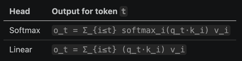
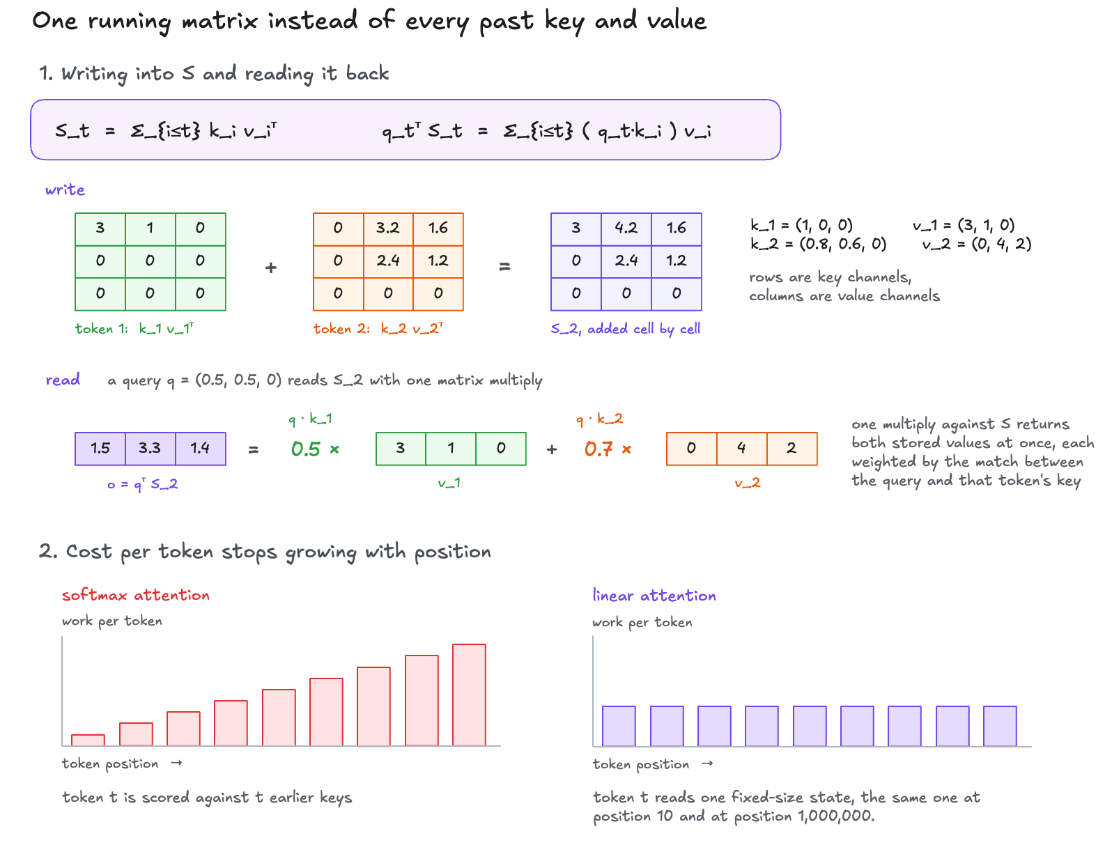
Each formula runs over every earlier position i, scores the current query q_t against the key stored at that position, and adds up the values v_i weighted by those scores. Softmax turns the raw scores into weights that sum to one by exponentiating each score and dividing by the total across all keys. The linear head skips that step and uses the raw dot product as the weight, so each earlier value is scaled by how well its key matches the current query.

Skipping softmax removes the need for the cache. Each term of the sum, (q_t·k_i) v_i, is a scalar times a vector, and the same term can be written as q_tᵀ (k_i v_iᵀ). The part in parentheses is the outer product of the two 128-long vectors, the 128×128 matrix whose entry at row a and column b is k_i[a] times v_i[b]. Multiplying q_tᵀ into that matrix computes the dot product q_t·k_i and multiplies v_i by that single number, which produces the same vector as the original term. Written this way, the query sits outside and the matrix depends only on token i, so each token’s matrix can be added into one running matrix S as soon as that token arrives, without knowing which query will later read it. The output is then q_tᵀ S, one matrix-vector multiply. Softmax blocks the factoring because its exponential and its division by the total both keep every weight tied to q_t.

S is one 128×128 matrix of numbers, and adding an outer product means adding it entry by entry. After t tokens the entry at row a and column b holds Σ_{i≤t} k_i[a] v_i[b], so the individual keys and values are not stored anywhere, only these 16,384 running sums.

The output stays exact because q_tᵀ S expands back into Σ_{i≤t} (q_t·k_i) v_i, the linear formula in the table above. Every read returns all the stored values at once, each scaled by how well its key matches q_t. Once the sequence passes 128 tokens, some keys have to overlap, so one token’s value never comes back by itself.

A softmax head scores token t against t earlier keys, so its work grows with position and the sequence total grows with the square of its length. A linear attention head does the same fixed amount of work at token ten and token one million.

Moonshot introduced KDA in Kimi Linear, a 48B-A3B hybrid model released in October 2025 to test the architecture at smaller scale. K3 uses a modified version of that operator, and the sections below cover both changes where the code shows them.

How KDA updates its state

KDA uses the same three 128-long vectors per head, with q_t and k_t normalized to unit length, and the same fixed-size recurrent matrix S. K3 sets the head dimension to 128 in its KDA layers, which is why q and k are 128 long and S is 128×128. The full layer also carries three fixed-size ShortConv caches, one each for the query, key, and value projections, which the diagrams below leave out.

The recurrence builds on regular linear attention. Linear attention keeps a state matrix S and adds one outer product per token, so old associations can interfere with new ones. DeltaNet treats S as associative memory trained by online gradient descent. It writes the difference between the value the state returns for key k_t and the value it should return. Gated DeltaNet adds a forget gate α_t, one number per token that multiplies the whole matrix so old entries fade with age. KDA turns α_t into 128 rates, one for each row of S. Inside one head, a row whose rate is near 1 keeps what it holds across the whole document, while a row with a smaller rate loses most of its contents within a few tokens. The 128 rates are not fixed. Each token computes its own set from its hidden state, on top of a learned bias that gives every row a default speed.

The Kimi Linear paper and K3 report write KDA as shown in the last row. A key channel is one of the 128 components of k_t. Each indexes a row of the 128×128 state, so decaying a channel scales that row. α_t contains 128 retention factors in (0, 1), one per key channel in FlashKDA's configuration, while β_t is a scalar write strength. Because α_t is a diagonal matrix rather than a number, its position relative to the erase term changes the result, while Gated DeltaNet's scalar gives the same state either way. KDA therefore decays first, then measures the erase step against the state a query would read.

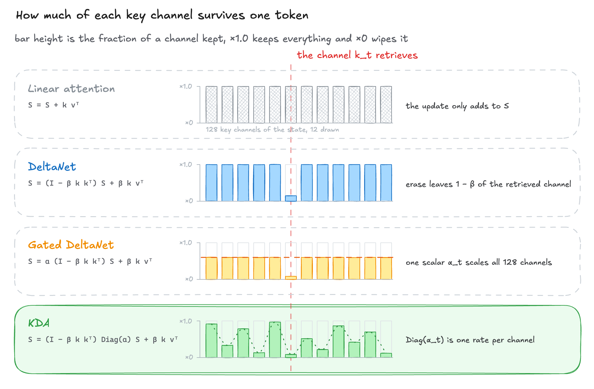
Each bar is one key channel of a head’s 128×128 state, and its height is how much of the previous state survives one token. Linear attention keeps everything, DeltaNet leaves 1 − β_t of the channel the incoming key retrieves, Gated DeltaNet fades all 128 at one rate, and KDA gives each channel its own rate.

Those retention rates cover only the first of three steps. A new token first decays the matrix and removes what its key already retrieves, then writes the incoming pair.

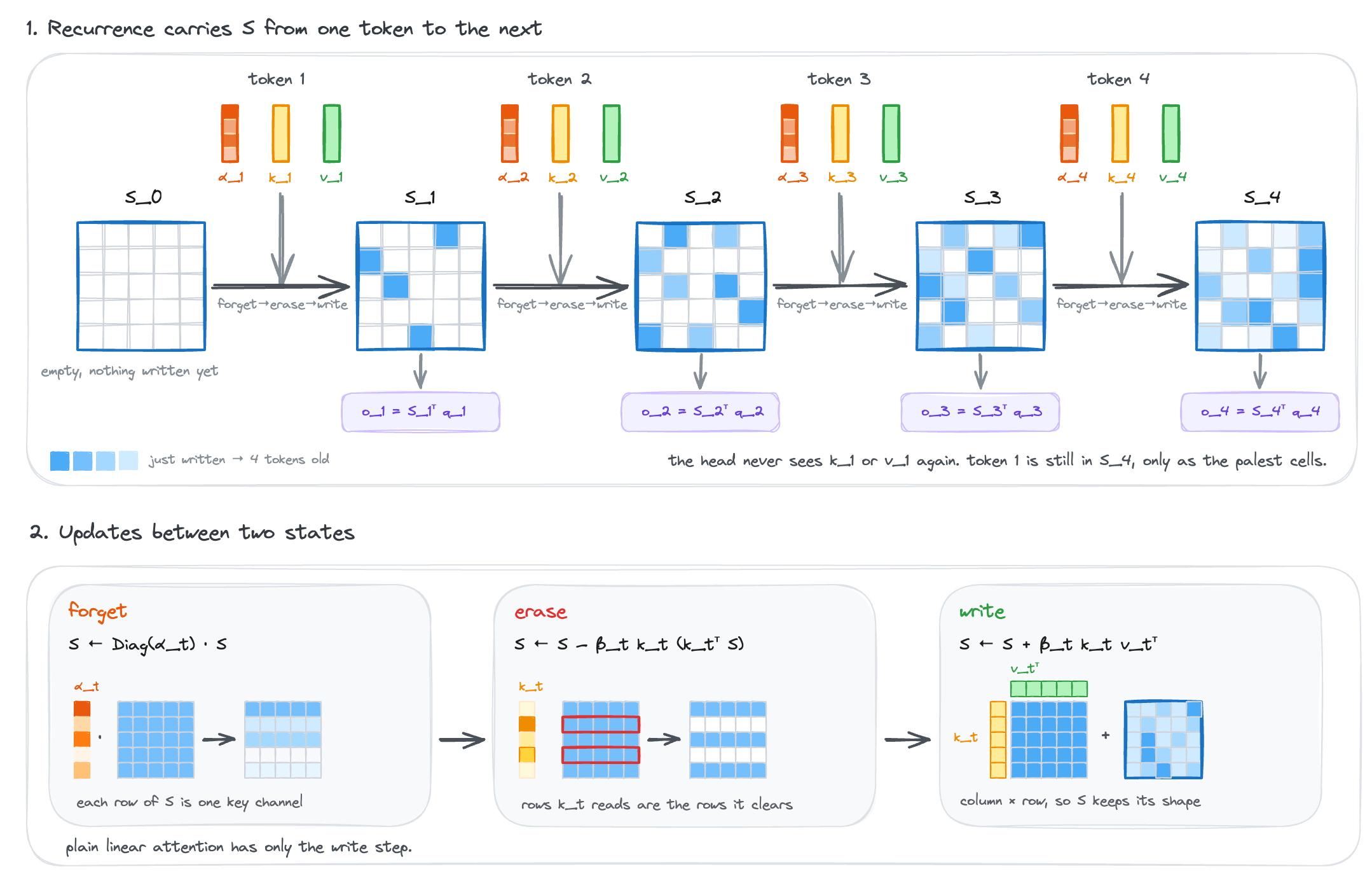
The two steps before the write remove different things. Forgetting handles age. S is fixed size and cannot retain everything across a million tokens, so stored information has to fade to leave room. Some of it also stops being worth keeping once a variable is reassigned, a subtask ends, or the topic changes. A gate controls what to forget, and tying it to the current token lets that decision change at each position. LSTMs added a forget gate for the same reason. A state that only accumulates cannot start fresh with the sequence. Decay also encodes recency, which lets the global attention layers later in this post drop positional encoding.

Erasing handles collisions between keys. Every token writes into the same matrix, so a key that resembles one written earlier reads back a mix of both values. The erase step, S ← S − β_t k_t (k_tᵀ S), takes the old part out before the new pair goes in. k_tᵀ S puts k_t where a query would go, and it returns the 128-long value the state currently gives back for that key. Multiplying the column k_t by that row builds a 128×128 matrix, and subtracting it removes the old association from each row of S in proportion to that row’s weight in k_t, so the channels the key does not address keep what they held. β_t scales how much comes out. Near 1 it clears the old value, and near 0 it leaves the value in place. The next read for k_t then returns what this token wrote instead of a sum over every similar key.

Decay applies to the key axis because that is the axis a query addresses. One axis of S is indexed by the 128 components of a key, the other by the 128 components of a value. Reading multiplies q_t into S along the key axis, so a query reaches the same components a key writes into. There is no separate query axis, and q_t is never stored because it appears only when the state is read. Fading a key row therefore weakens what arrived under keys pointing in that direction. Fading a value column instead would shrink the same coordinate of every stored value no matter which key wrote it, which changes the output scale rather than forgetting anything. The reference kernel shows the shapes. S is [B, HV, K, V] and the decay gates g are [B, T, HV, K], where B is the batch, T the number of tokens, HV the number of value heads, and K and V the key and value head dimensions. Every head gets one gate per key component at every token, while S has no T axis because the same matrix is carried forward.

The recurrence ships in flash-linear-attention, an open source library of linear attention kernels, as fla.ops.kda. FLA’s reference implementation is forget, erase, write, and read in three lines.

flash-linear-attention/fla/ops/kda/naive.py

for i in range(0, T):
    q_i, k_i, v_i, g_i, b_i = q[:, i], k[:, i], v[:, i], g[:, i], beta[:, i]
    S = S * g_i[..., None].exp()
    S = S + torch.einsum('b h k, b h v -> b h k v', b_i[..., None] * k_i, v_i - (k_i[..., None] * S).sum(-2))
    o[:, i] = torch.einsum('b h k, b h k v -> b h v', q_i, S)

The first line forgets by scaling S with g_i[..., None].exp(), which is α_t because g holds decay in log space. The second combines erase and write, where v_i - (k_i[..., None] * S).sum(-2) is the gap between what S currently returns for k_i and the target value. The third reads. Work per token is constant, so total cost is linear in sequence length.

α_t comes from a per-head low-rank projection that produces one decay logit per key channel, and how that logit becomes a decay matters for the kernel work later. Kimi Linear’s version is naive_kda_gate, which sits directly above the K3 replacement in gate.py, documented as g = -A_log.exp().unsqueeze(-1) * softplus(g + dt_bias.view(g.shape[-2:])). Softplus has no lower bound, so one step can decay a channel to nearly zero. K3 replaces it.

flash-linear-attention/fla/ops/kda/gate.py

def naive_kda_lowerbound_gate(
    g: torch.Tensor,
    A_log: torch.Tensor,
    dt_bias: torch.Tensor | None = None,
    lower_bound: float = -5.0,
    output_dtype: torch.dtype = torch.float32,
) -> torch.Tensor:
    H, _ = g.shape[-2:]
    g = g.float()
    if dt_bias is not None:
        g = g + dt_bias.view(H, -1)
    g = lower_bound * F.sigmoid(A_log.view(H, 1).exp() * g)
    return g.to(output_dtype)

Sigmoid returns a value in (0, 1) and lower_bound is negative, so g always lands between −5 and 0. The state is scaled by exp(g), which therefore stays between exp(-5) ≈ 0.0067 and 1. A channel can still lose almost everything it holds, but never all of it in a single token. The layer exposes the choice as safe_gate, documented as letting the kernel assume gate values lie in [lower_bound, 0) and use M=16 TensorCore acceleration. The kernel section later shows what that assumption enables.

Kimi Linear measured the 128 rates against a single rate on three synthetic tasks, reproducing a palindrome, recalling the value for one of many keys, and tracking a LIFO stack. Each one requires the model to drop stored items at points the input decides. KDA matched or beat Gated DeltaNet, which fades all 128 channels at one rate, at every training length from 256 to 2,048 tokens, and on the first two it reached full accuracy in about a third of the training steps. Mamba2 decays its state but has no delta rule, so nothing removes an old association before a new one is written. By 1,024 tokens it scores zero on all three.

KDA belongs to the Diagonal-Plus-Low-Rank family, S_t = (D_t − a_t b_tᵀ) S_{t-1} + k_t v_tᵀ, where D_t holds the 128 decay rates on its diagonal and a_t b_tᵀ is the erase term. A general kernel for this family carries a_t and b_t as independent vectors and pays for extra matrix multiplications in the chunk math. KDA sets both to k_t, which the erase step already loads, and Kimi Linear measures roughly twice the operator efficiency of a general DPLR implementation.

Three KDA layers and one MLA layer

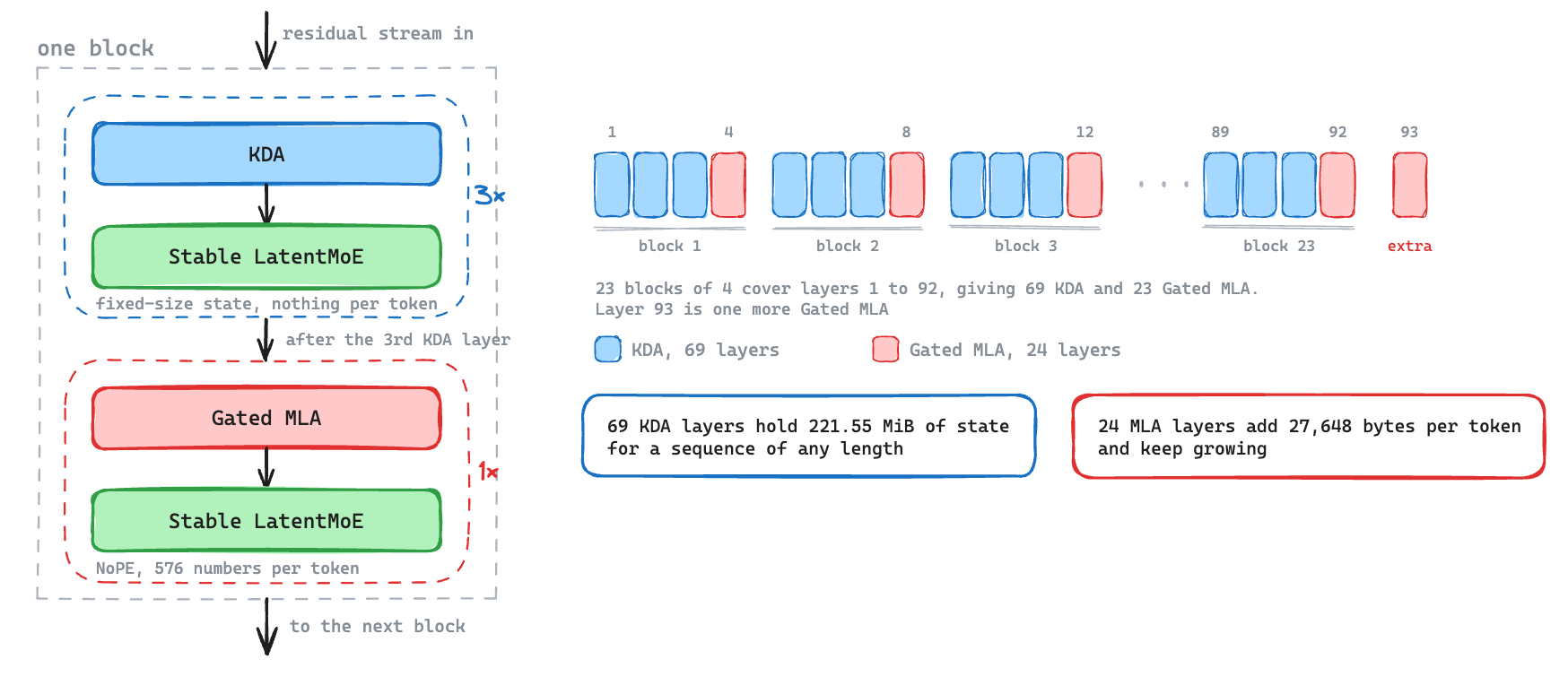
Per-channel decay slows the loss, but a fixed-size state still cannot return an exact token from far back, so K3 keeps some full attention. Each block stacks three KDA layers and one Gated MLA (Multi-head Latent Attention) layer, a 3:1 ratio across 93 layers. The pinned config.json lists the 24 full attention layers by index. They appear every fourth layer, and one extra at the end makes the final layer global. Every attention layer except the first feeds a Stable LatentMoE feed-forward layer. The first layer keeps a dense feed-forward network, set by first_k_dense_replace in the config. Attention Residuals (AttnRes) let each layer attend over preceding block outputs instead of relying on one compressed residual stream.

How MLA compresses the cache

MLA comes from DeepSeek-V2. It applies ordinary softmax attention over a compressed cache. Instead of keeping one key and value per head per token, it projects the token into one latent vector shared by every head, caches that vector, and rebuilds each head’s key and value when the layer runs. K3 sets kv_lora_rank to 512 and qk_rope_head_dim to 64, so one MLA layer holds 576 numbers per token, or 1,152 bytes in bf16. For comparison, ordinary multi-head attention would store a separate 128-long key and value for each of the 96 heads, 49,152 bytes for the same token and layer. MLA compresses the cache about 42 times before KDA removes anything (49,152 / 1,152 ≈ 42.7).

What the hybrid saves

A KDA layer holds 96 recurrent matrices of 128×128 and three ShortConv caches with a kernel size of 4. Assuming bf16 for both, the recurrent matrices use 3 MiB per layer and the convolution caches add 216 KiB. Across 69 layers, the fixed cache is 221.55 MiB for a sequence of any length. The 24 MLA layers still grow at 24 × 1,152 = 27,648 bytes per token. The relevant comparison is the same model with all 93 layers built as MLA, the design K3 replaced, rather than an uncompressed baseline.

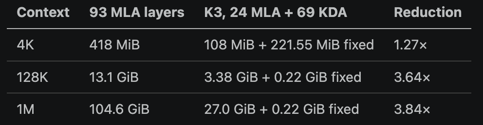
The reduction cannot exceed 93/24, about 3.9 times, because the MLA layers keep growing with every token. K3’s MLA portion adds 27 KiB per token instead of 105 KiB for 93 MLA layers. The 221.55 MiB KDA cache is allocated from the first token. The 69 MLA layers it replaces would have cost 79,488 bytes per token, so the hybrid uses more memory than an all-MLA model below roughly 2,923 tokens. The 221.55 MiB is charged per request, not per model, so it multiplies with concurrency rather than amortizing across it.

These totals are a bf16 lower bound. FlashKDA accepts bf16 or fp32 recurrent states, while vLLM’s KDA cache calculator uses fp32 for the recurrent matrix. A runtime that keeps S in fp32 pays more than the table above shows.

896 experts per layer, 16 active

What is an expert?

An expert is a feed-forward network, a small stack of weight matrices with nonlinearities. It is the same component that follows attention in every dense transformer. Despite the name, an expert is not an agent, not a layer of the stack, and not a model trained on its own. A dense transformer runs one such network on every token. A Mixture-of-Experts layer holds many copies and routes each token to only a few. Backpropagation trains every expert weight from the first pretraining step, and post-training keeps updating them. Unlike a dense network, an expert receives gradients only from tokens routed to it, so load balancing across experts is important.

The router is a small linear layer that scores every expert for the incoming token, and the highest k scores win. Each K3 MoE layer has 896 routed experts and activates 16. Two shared experts run on every token, and their output joins the routed path’s output. Each of the 92 MoE layers carries its own pool, so E1 in one layer and E1 in the next are different networks.

Splitting experts into shared and routed comes from DeepSeekMoE. Some transformations apply to nearly every token. If they live only in routed experts, each expert must encode them because a token sent to E5 cannot use E2. This duplicates the same function across many of the 896 copies, consuming parameters that could hold specialized behavior. A shared expert sees and receives gradients from every token, so common work tends to settle there during training. Routed experts then do not need a separate copy because the shared experts run regardless of which 16 the router picks. It is a training bias, not a constraint, because the code does not enforce this division.

This separates K3’s 2.78T total parameters from its 104.2B activated per token. Capacity grows with the pool, while per-token arithmetic grows only with the selected experts.

K3 also projects the 7,168-wide hidden state down to 3,584 before the router runs, so the routed experts read and write half-width vectors while the shared experts stay at 7,168.

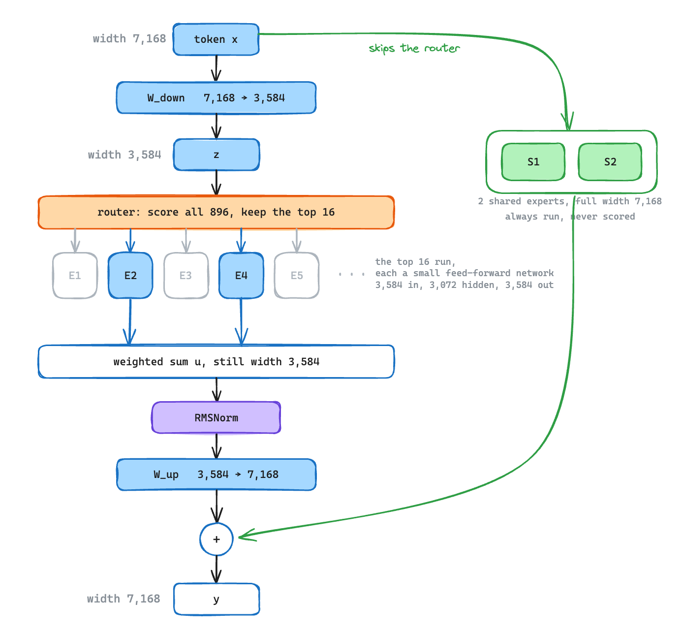
GPU communication and expert weight traffic scale with routed width, so halving it to 3,584 makes a pool of 896 affordable. K2 had 384 routed experts at the full 7,168 width, with 8 active, one shared expert, and no latent projection.

Routing 16 of 896 breaks the standard design in two ways. To control exploding activations, K3 places RMSNorm between expert aggregation and the up-projection because the routed path composes roughly four consecutive matmuls without a scale bound. It also adds SiTU-GLU, which applies a smooth softcap β·tanh(x/β) to both factors of the SwiGLU product. β is 4 on the gate branch and 25 on the up branch, bounding output at 100 while preserving the SwiGLU shape near the origin.

The second failure is routing collapse. An expert’s load is the number of tokens routed to it during a step, and the top-k rule does not keep loads even. A few experts win most scores and receive most gradients, making them more likely to win next time. Others receive nothing and stop learning. Balanced loads also improve speed because experts are spread across GPUs and the busiest one sets step time.

DeepSeek-V3-style auxiliary-loss-free balancing adds a bias to each expert’s router score before top-k. After each step, an overloaded expert’s bias falls by a fixed amount γ, while an underloaded expert’s bias rises by the same amount. The fixed step contains no information about the size of the load error. With nearly a thousand experts, the bias either overshoots and oscillates or approaches the right value too slowly.

Quantile Balancing (QB) computes a next-step bias from one batch’s router scores. The router takes Top-(k+1) over the currently biased scores. The first k entries are the routes, while entry k+1 supplies the cutoff α_i. For expert j, QB forms the raw margin s_i,j − α_i. If the target is q tokens, the negative of the (q+1)-th largest raw margin leaves exactly q margins above the threshold when the cutoffs are held fixed and there are no ties. QB computes this value for every expert, mean-centers the biases, and applies them on the next step.

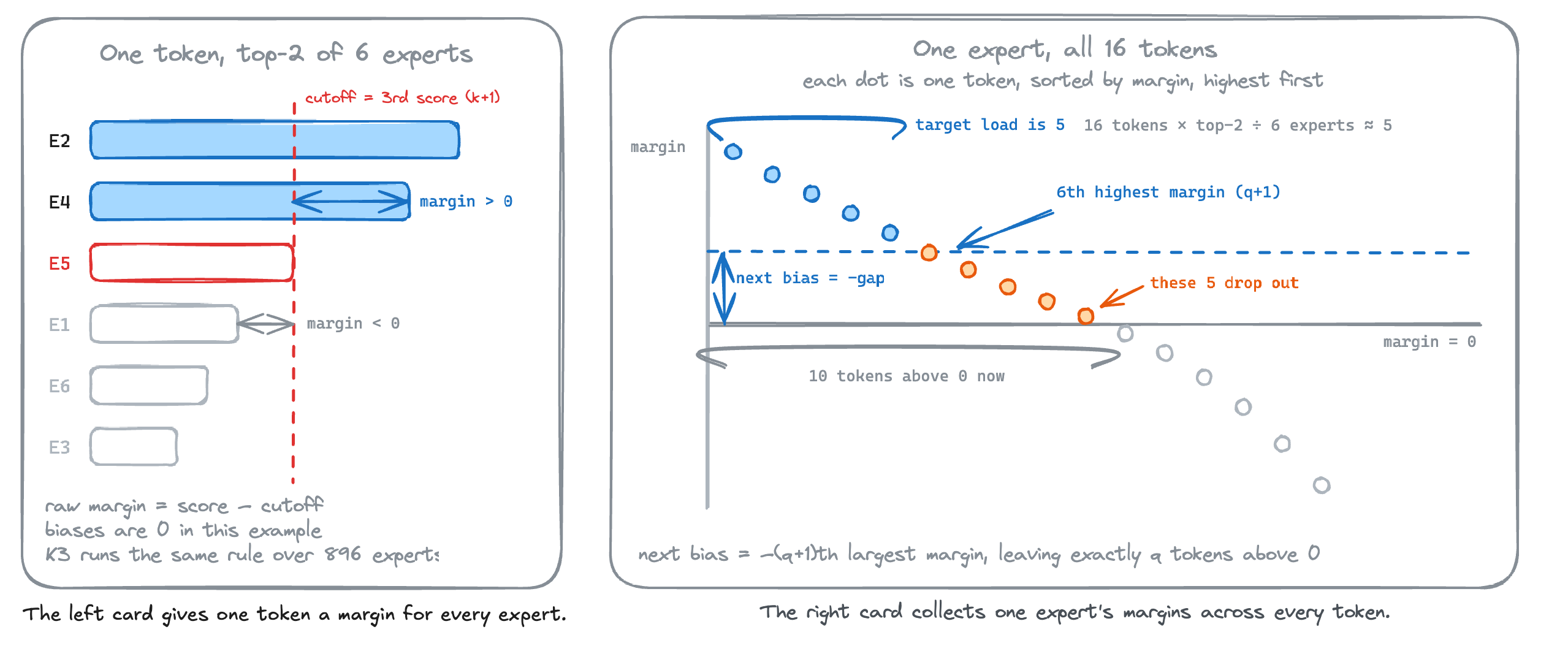
Balanced routing is an assignment problem, one that sends each token to its highest-scoring experts while every expert receives exactly q tokens. Problems of that shape are solved by putting a price on each expert. At the correct price, exactly q tokens still find the expert worth picking, and the router bias acts as that price. The old sign update searches for the correct price in fixed steps of γ, while QB computes it from one batch’s margins in a single pass.

At training scale, the exact quantile would require gathering millions of margins, so QB uses a histogram. One integer all-reduce sums each expert’s per-GPU bin counts, a few hundred bins per expert per step, and the pooled counts estimate the quantile up to the bin width. The bias freezes at inference, leaving an ordinary top-k router during serving.

FlashKDA steps the state once per 16 tokens

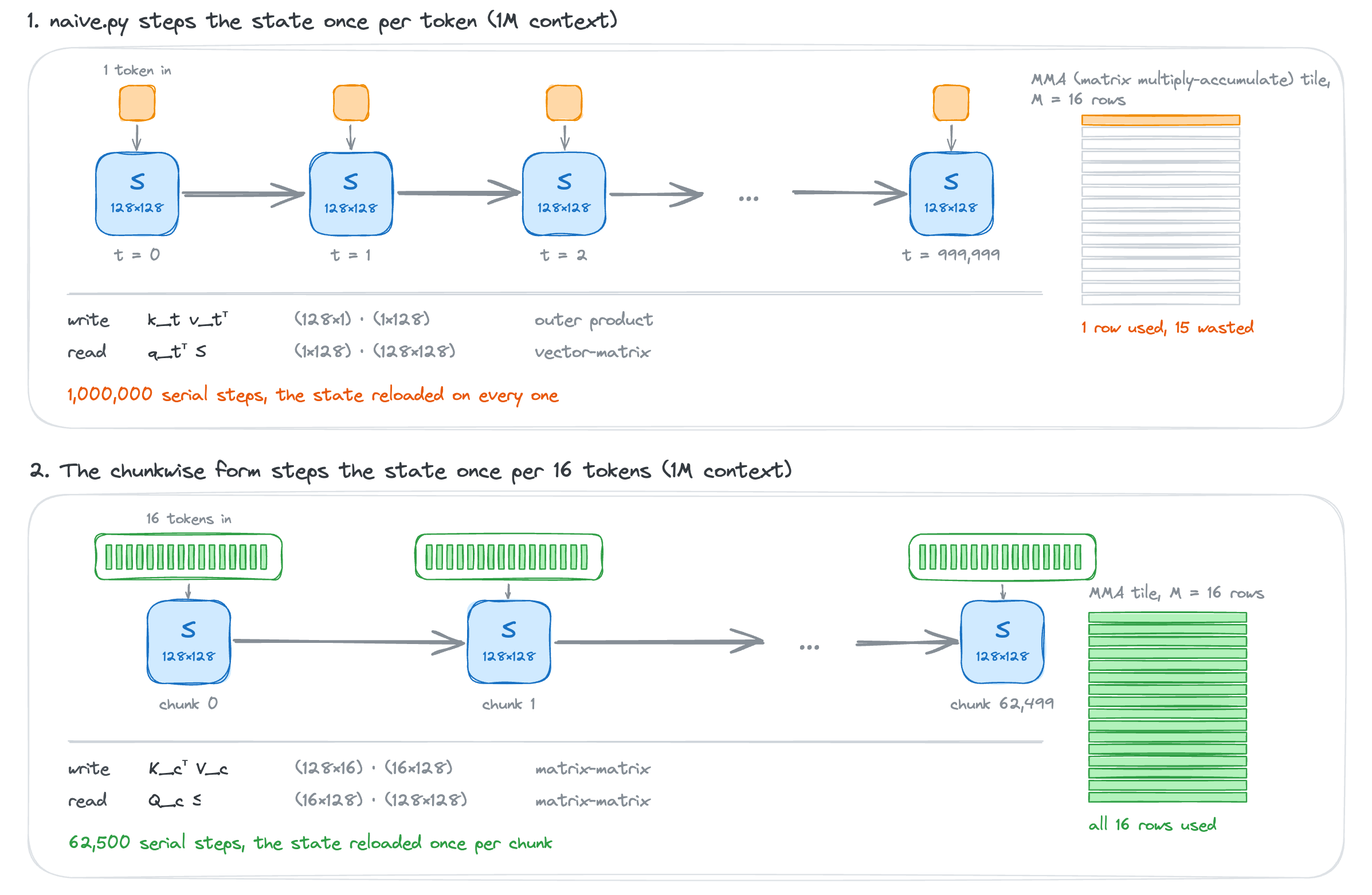
FlashKDA implements KDA’s chunkwise forward pass for training and inference prefill in CUTLASS (NVIDIA’s template library for writing custom GPU matmul kernels that still reach Tensor Core throughput). The naive.py loop steps once per token, requiring a million serial matrix-vector steps on a 1M-token sequence without reaching a Tensor Core. A Tensor Core is the dedicated matrix-multiply unit inside each streaming multiprocessor, and it accepts only matrix-by-matrix work. On an H100 it delivers about 990 TFLOPS of BF16 against roughly 67 TFLOPS of FP32 on the general-purpose CUDA cores. A single token updates the state with an outer product and reads it back with a matrix-vector product, and neither shape fills a Tensor Core tile, so the loop falls back to the slower cores and reloads the whole 128×128 state for every token.

The chunkwise form splits the sequence into fixed-size blocks, 16 tokens here. It steps the state once per block and computes tokens within a block together as dense matmuls, which gives the products a second matrix dimension large enough to fill a Tensor Core tile. The state now loads once per 16 tokens, and the serial chain on a 1M-token sequence drops from a million steps to 62,500. The result matches the token loop. Only the hardware schedule changes. Chunk-local math runs in parallel over every token in the batch, while state recurrence is serial per sequence. A single fused kernel makes the parallel work wait for the serial work. The repo’s deep-dive doc reports that splitting the phases gave at least a 15% end-to-end speedup over the fused prototype.

FlashKDA/csrc/smxx/fwd_launch.cu

// ===== Launch Kernel 1 (prepare) =====
constexpr int kK1Threads = 256;
dim3 grid_k1(total_tiles, H);
kernel1<<<grid_k1, block_k1, smem_size_k1, stream>>>(/* ... */);

// ===== Launch Kernel 2 (recurrence) =====
constexpr int kK2Threads = 32 * 2 + 128;
dim3 grid_k2(N, H);
kernel2<<<grid_k2, block_k2, smem_size_k2, stream>>>(/* ... */);

Kernel 1 launches one CTA (cooperative thread array, the group of threads that runs on one streaming multiprocessor and shares its memory) per 16-token chunk per head, computes each chunk’s local matrices at full occupancy, and writes them to a workspace. Kernel 2 launches one CTA per sequence per head, with four MMA warps plus a load warp and a store warp, and walks the chunk recurrence serially. The 128×128 state stays in shared memory in bf16 for the sequence, with updates using fp32 FMA before casting back. The split gives the token-parallel stage and the head-parallel recurrence separate launch shapes, so each is scheduled and tuned on its own.

K3’s decay change simplifies the tile math. Intra-chunk work rescales keys by reciprocal cumulative decay. Because each retention factor is in (0, 1), the reciprocal can overflow in finite precision. Kimi Linear handled this by computing diagonal 16-token tiles with explicit position-pair arithmetic, making those tiles the intra-chunk bottleneck. The lower-bounded sigmoid gate above keeps every retention factor above exp(-5) ≈ 6.7×10^−3. Rescaling stays inside BF16 range, so diagonal tiles need no special path and every tile becomes a dense Tensor Core matrix multiply. The bound reaches the kernel as one host-folded constant.

FlashKDA/csrc/flash_kda.cpp

float gate_scale = float(lower_bound * 1.4426950408889634);

The multiplier is log2(e), which prepares the bound for the kernel’s base-2 exponentials.

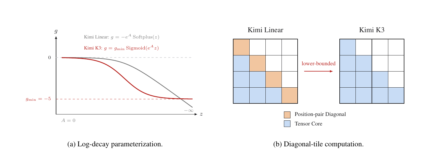
Figure 3 from the report. Left, the bounded log-decay curve against Kimi Linear’s unbounded negative-Softplus. Right, the tile consequence. The orange position-pair tiles disappear.

The chunk size is 16 rather than flash-linear-attention’s default of 64 for three reasons. Bounded decay keeps a 16-token chunk’s cumulative products inside bf16, which removes the intra-chunk rescaling that larger chunks need. A 16×16 matrix inverse is cheap enough to compute as a Neumann series, exact after three doubling rounds because the matrix is strictly lower triangular. And every piece of the chunk math maps onto SM80 MMA (matrix multiply-accumulate) instructions, so the kernel stays portable across GPU generations instead of depending on Hopper-only matrix instructions. The complete implementation still requires SM90 or newer. The build list in setup.py starts at Hopper, and the load and store paths use Hopper-generation TMA and STSM instructions.

The open repo is forward-only prefill with a fixed head dimension of 128, auto-dispatched as an FLA backend under torch.inference_mode() when the inputs are bf16 and safe_gate is on, so the bounded gate from earlier is a precondition for the fast path. The backward pass, the decode kernel, and the SM-level context-parallel planner stay closed.

Every GPU gets exactly S × K tokens at every step

With 896 routed experts, router imbalance affects infrastructure as well as training quality. Quantile Balancing evens aggregate expert loads, but routing can still skew within one step. In conventional expert parallelism, which DeepSeek’s open-source DeepEP library implements, each GPU (a rank) holds a slice of the 896 experts and receives whatever tokens the router assigned to that slice. Token counts differ across ranks, so the busiest rank sets step time and the varying activation shapes fragment memory. MoonEP sends every rank S × K tokens per step regardless of routing skew, where S is tokens per rank and K is the top-k.

Dynamic redundant experts make this possible. When an expert overflows its home rank, the planner duplicates it onto an underloaded rank for that step. Duplicating means a prefetch kernel copies the expert’s full weights over NVLink into one of a few spare weight slots each rank reserves, and the two copies of the expert each process part of its tokens. The report proves that a balanced plan always exists with at most E/R redundant experts per rank. ECHO and UltraEP preset redundancy and can stall when no feasible plan fits the cap. The balancing step of MoonEP’s planner is a greedy transfer loop that runs in a single warp (a group of 32 GPU threads) and keeps its balance array in registers throughout, touching memory only to read the initial token counts and to record each move.

MoonEP/moonep/planning.py

# balance stays in registers throughout: lane holds
# bal[j]=group_tokens[lane+j*32]-CAP, CHUNK=ceil(R/32).
while keep_balancing:
    surplus, surplus_rank = reg_scan_argmax_min_idx(balance, R, lane)
    deficit, deficit_rank = reg_scan_argmin_min_idx(balance, R, lane)
    if surplus <= 0 or deficit >= 0:
        keep_balancing = False
    else:
        # The move amount is limited by the receiver's
        # shortfall; refill deficit_rank back to CAP in one shot.
        move_tokens = -deficit
        ...
        z_tensor[surplus_rank, deficit_rank] = move_tokens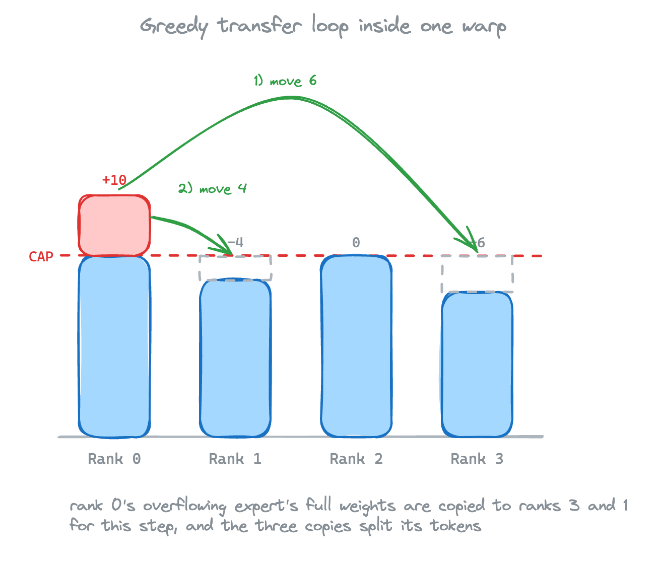

A second mechanism reduces traffic. When a token’s top-k entries route to multiple experts on the same destination rank, only one copy crosses NVLink. Each routing entry stores the offset where the token will be written on its destination rank. For entries whose destination rank already appears earlier in the same token’s list, the kernel stores the negated offset instead, and the send path skips the payload for any entry with a negative value.

MoonEP/moonep/planning.py

# ... the first entry per destination rank stays non-negative and carries
# the payload; later entries encode -raw_dst - 1 and only carry weights.
for k in cutlass.range_constexpr(K):
    d = dests[k]
    dup = ...            # register bitmask of ranks already seen for this token
    if dup:
        dst_out[base_idx + k] = -(dst_vals[k]) - 1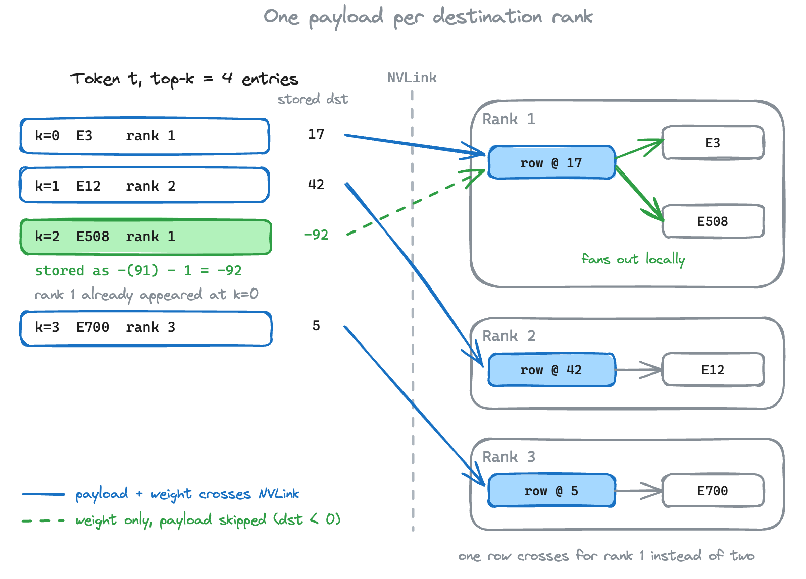

The payload is the token vector itself, the 3,584 numbers the expert will multiply, about 7 KB in bf16. The weight is the router’s score for one (token, expert) pair, a single fp32 number, 4 bytes. Neither term means the expert’s weight matrices, which never leave their home rank. When a token routes to two experts on the same rank, the rank needs the token vector only once. The first entry carries it, and the rank copies the row locally for the second expert. The score cannot be shared the same way. Combine multiplies each expert’s output by that expert’s own score, and the router gave the two experts different scores, so the second entry still carries its 4 bytes while skipping the 7 KB row. The sign of the stored offset works as a flag. The send path skips the payload for any negative entry, the receiving rank copies the one row it did get to its other experts, and the combine phase sums the expert outputs in fp32. Both libraries reduce dispatch traffic. DeepEP makes each row smaller by quantizing it to FP8. MoonEP sends fewer rows at full precision.

Guaranteed balance simplifies the stages after dispatch. Every rank receives exactly S × K rows, and each row lands directly in a slot grouped by expert, so the receive buffer is a fixed allocation of S × K rows and a few padding slots. DeepEP has to size its buffer for the worst case where all R ranks route every token to the same rank, which is S × K × R. In MoonEP the rows arrive already grouped by expert and the buffer shape never changes, so the expert GEMM reads the buffer directly and the CPU launches each layer without waiting for the GPU to report token counts. The C++ code is 478 lines of memory management. Every GPU kernel, including the planner, is written in Python through the CUTLASS CuTe DSL.

Post-training distills nine RL models into one

The pipeline runs SFT, RL, and then distillation. RL trains nine complete models, one for each pairing of three domains (general, agentic, and coding) with three reasoning-effort levels. They are unrelated to the architecture’s MoE experts.

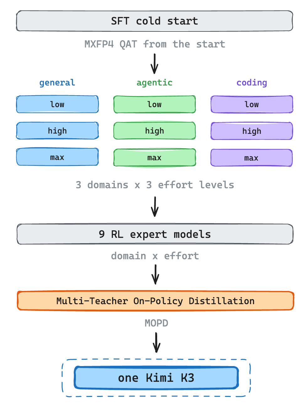
Reasoning effort is trained with a per-problem token budget and a reward of −1 for exceeding it. RL starts at the maximum budget, and annealing the budget downward produces the lower-effort models.

The distillation stage is MOPD, Multi-Teacher On-Policy Distillation. Teacher and student are knowledge-distillation terms, not RL terms. The nine RL-trained models are the teachers, and the student is the single final model that absorbs all of them. Classic distillation trains the student to imitate text the teacher generated. In MOPD the student generates its own rollouts, and each token receives a reward from the clipped log-ratio between the student’s probability and that of the teacher matching the rollout’s domain and effort. Distillation therefore runs on the same RL infrastructure, partial rollouts included, instead of needing a separate imitation-learning pipeline.

The RL environments make two useful design choices. The agent harness is a white-box collection of configurable modules for tools, system prompts, context management, skills, memories, and subagents. It can instantiate Kimi Code, Claude Code, Codex, OpenClaw, or Hermes. The report says different task groups use different harness configurations, exposing the model to varied scaffold combinations. The reward systems also assume the model will cheat. The GPU-kernel suite scores correctness and speed against expert implementations while penalizing CUDA-graph replay, input caching, and precision reduction. Web development tasks receive zero reward when a project fails to build or fakes the artifact.

The report says co-located RL keeps a 1M-context experiment within a few hundred GPUs, helped by the fixed-size KDA state and by offloading evicted cache blocks to CPU DRAM. At 1M tokens, rollout lengths vary widely. Generation pauses after a fraction λ of trajectories completes, and unfinished trajectories resume in the next iteration. Per-token regularization absorbs the resulting off-policyness. This requires nearly free environment pauses, which AgentENV provides.

AgentENV pauses the world while the model thinks

AgentENV is a Rust sandbox runtime built on Firecracker microVMs (AWS’s KVM-based virtual machine monitor, built for Lambda, that boots minimal VMs in about 125 ms with under 5 MB of overhead each). It is open-sourced under kvcache-ai and, according to the report, developed “in collaboration with our partners.” Its README says it powers agentic RL training for K3, but the repo contains no RL code. It exposes an E2B-compatible HTTP API that an external RL loop drives.

During K3’s training, each agentic rollout runs its commands inside a sandbox, and the report maps the lifecycle operations onto RL needs. Pause suspends the environment of a trajectory the partial-rollout scheduler set aside. Fork gives reward judging a disposable copy of a finished sandbox, so scoring cannot leave side effects in the original. Snapshot supports recovery when an environment fails.

Container-based sandboxes suffered kernel panics and deadlocks from aggressive agents. K3 therefore uses VMs in which an agent can mount disks, run containers, or launch nested VMs without sharing the host kernel. Training and evaluation created 51,219,741 sandboxes across 1,505,678 images.

The report gives checkpoint and resume times of 133 ms and 49 ms, with a paused sandbox consuming zero CPU and memory. Model inference can account for ~98% of a sandbox’s lifetime, so pause and resume speed affects fleet cost. Three mechanisms produce those numbers.

A disk snapshot avoids copying the upper layer’s data. Sandbox disks are overlaybd layered images with one writable upper layer. Snapshotting seals and renames that layer, then stacks a fresh empty upper layer on top. The rename is constant-time, but sealing first flushes pending writes, scans the mappings, and appends a compact index. That work can grow with the number of written mappings.

AgentENV/storage/overlaybd/src/image/image_file.rs

let (reopened, descriptor) = current.close_seal_and_reopen().await?;
lower_files.extend(reopened.get_lower_files());

tokio::fs::rename(&upper_data_path, output_layer_path)
    .await
    .with_context(|| { /* ... */ })?;

prepare_runtime_upper(&upper_data_path, upper_index_path.as_deref(),
                      virtual_size, upper_mode)
    .context("prepare fresh upper after restack")?;

The default direct memory-snapshot path skips an intermediate file. With direct_overlaybd=true, AgentENV first takes a state-only snapshot, which saves the CPU and device state but leaves the guest’s memory out. For the memory, it asks Firecracker which pages the guest has written since the last checkpoint, so unchanged pages are not copied at all. It then reads only those changed pages straight from the running VM’s memory with process_vm_readv, a Linux call that lets one process read another process’s memory, and packs them into a sealed overlaybd layer without writing a memory file in between. A supported fallback writes mem.bin and converts that sparse file afterward. The /vm/dirty-memory-ranges query does not exist in upstream Firecracker. The patched API spec is in firecracker.yaml.

AgentENV/src/sandbox/firecracker/sandbox.rs

let firecracker_pid = self.fc_instance.pid()?;
self.fc_instance.create_state_only_snapshot(vm_state_path).await?;
let dirty_ranges = self.fc_instance.get_dirty_memory_ranges().await?;
convert_dirty_memory_to_overlaybd(firecracker_pid, &dirty_ranges, &mem_overlaybd_dir)
    .await
    .context("convert dirty memory ranges to overlaybd layer")

Resumed siblings share one memory device. The memory snapshot becomes a read-only ublk block device that Firecracker maps copy-on-write. The device manager reference-counts devices per image, so N sandboxes forked from one template share one device and host page-cache population. Combined with guest-side balloon and DAMON reclaim, this supports the report’s claim of up to 6.5× memory overcommit.

AgentENV/src/sandbox/ublk/device.rs

/// Shared memory devices are read-only overlaybd devices that can be
/// used by multiple sandboxes simultaneously. When multiple sandboxes
/// boot from the same snapshot template, they share a single ublk
/// device (and thus the same Linux page cache).
if let Some(weak) = self.shared_mem_devices.get(&key) {
    if let Some(strong) = weak.upgrade() {
        return Ok(SharedMemDevice { inner: strong });
    }
}

Fork uses the same pieces. The source pauses and resumes while N children boot concurrently from its snapshot. Each succeeds or fails independently, letting the RL system judge rewards without changing the live trajectory. The tree retains an excluded uffd-core userfaultfd implementation as an alternative reference. The active restore path uses ublk, but the public history does not establish which design came first.

KDA states and MLA KV blocks share one paged pool

Serving mixed KDA and MLA layers requires two cache types. MLA’s KV cache grows per token, while each KDA layer keeps a fixed-size recurrent matrix and three ShortConv caches per request. A cached prefix is reusable only when both can be restored at the same boundary. K3 packs KDA states into the same paged pool as MLA KV blocks but caches the two at different granularities. Prefix matching hashes the token stream in 512-token blocks, and several hash blocks fit inside one larger physical memory block. The MLA KV cache holds an entry for every token, so it can be restored at any 512-token boundary. The KDA state cannot, because each new token overwrites it in place. K3 therefore saves a copy of the state, a checkpoint, at only some of the boundaries. A lookup runs in two stages. It first finds the longest prefix whose hash blocks match, then takes the latest boundary inside that prefix that also has a KDA checkpoint, and prefill resumes from that point.

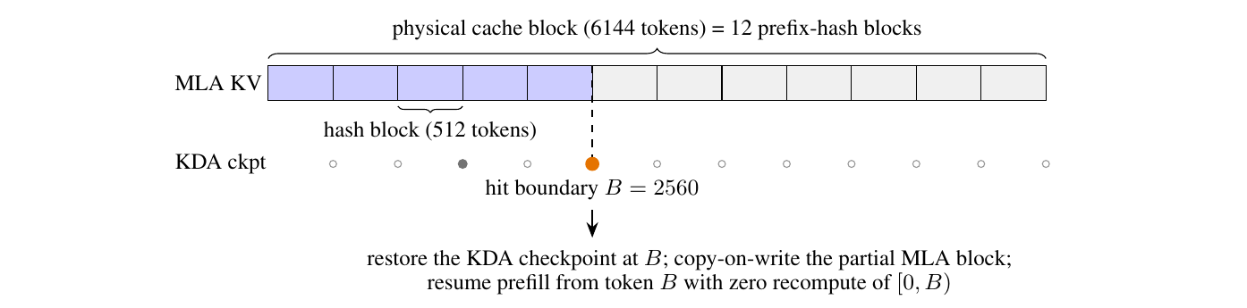
Figure 12 from the report. One 6144-token physical block holds twelve 512-token hash blocks. The matched prefix ends at token 2560, where a KDA checkpoint also exists, so prefill resumes there and recomputes nothing before it.

The report’s example is a typical coding request at 1M context, which arrives with a 400K-token prefix from earlier turns and adds only 4K new tokens. On a cache hit the server prefills the 4K new tokens. On a miss it re-prefills the whole 400K-token prefix. The fleet layer routes each session to the cluster holding its prefix cache, since moving the request is cheaper than moving the cache. Consistent hashing assigns a secondary cluster across the fleet. Budget-based admission control prevents million-token bursts from starving short requests, whose costs differ by three orders of magnitude.

Results and gaps

The report’s own summary of the whole program is a 2.5× efficiency gain over Kimi K2 at matched validation loss, attributed jointly to the architecture, data, and recipe changes.

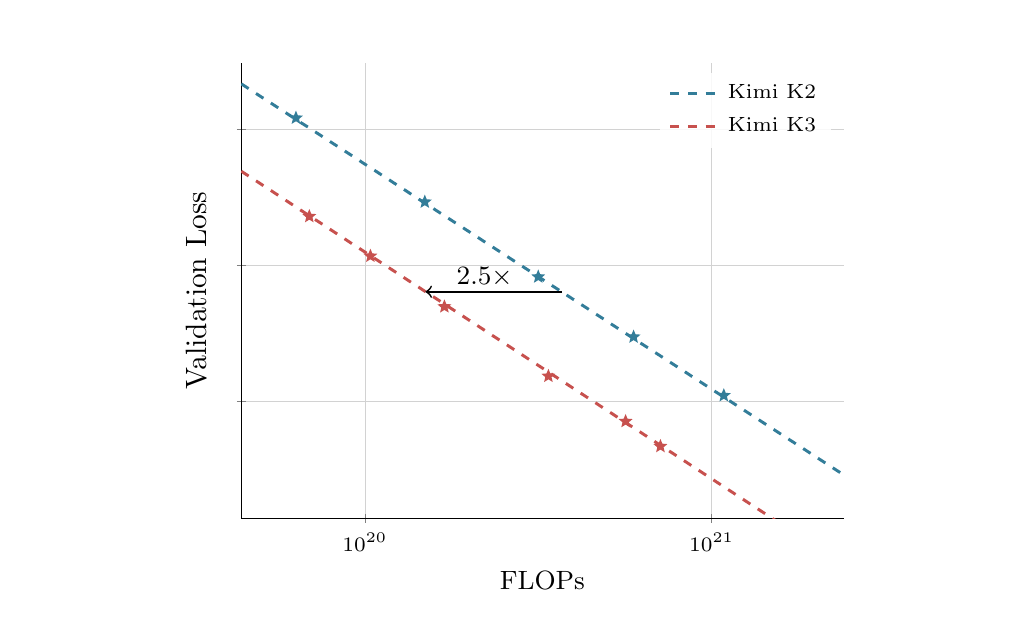
Figure 7 from the report. Fitted scaling-law curves for both models. K3 reaches K2’s validation loss with 2.5× fewer training FLOPs.

One benchmark tests the attention decision directly. K3’s standard BrowseComp run compacts the context once it passes 300K tokens and scores 91.2. A second run turns compaction off and lets the context grow to the full 1M window, and the score drops only to 90.4. Staying accurate over a raw 1M-token context is the intended benefit of a fixed-size attention state. The report also identifies a weakness. On the research-level reasoning benchmarks HLE-Full and CritPt, K3 trails both frontier labs by wide margins.

The release documents several reusable design patterns. A fixed-size recurrent state simplifies checkpointing, context parallelism, and prefix caching. Histogram-estimated quantiles drive expert load balancing. Varied harness configurations expose agents to different scaffolds. MicroVM checkpointing makes long inference waits cheap, while forks isolate reward judging from live trajectories.